The Joy of Secs: Part 1

One of the most widely deployed asymmetric cryptographic algorithms used today (driven by the popularity of blockchain technology) is based on elliptic curves over finite fields. Like all good engineers I struggled to just accept how they work. I needed to dig deeper to better understand the mathematics and in doing so decided to share my experience ...

This post ended up being a lot longer (in length and "the making") than I intended and so I've broken it in to parts. In this post we'll cover the basics of Finite Fields. You can also read part 2 about more advanced operations and non-prime Finite Fields and part 3 which covers calculations on elliptic curves.

So why The Joy of Secs? Well today we’re going to focus on two particular curves that are defined by the Standards for Efficient Cryptography Group, namely secp256k1 and secp256r1. The former is widely used in blockchain platforms and the latter is the NIST prime 256 curve, commonly available in hardware on mobile platforms. For those with a penchant for details, both of these curves are considered to have weaknesses, the SafeCurves website has a wealth of information on why.

I set myself two goals:

1. Be able to calculate $y$ given $x$ for a particular curve (this will help us to understand the format of an Elliptic Curve public key)
2. Understand how point addition works (this will help us to understand what an Elliptic Curve private key represents and how to derive a public key for a given private key)

Before we dig in to the elliptic curve side of things we firstly need to understand what “defined over a finite field” means. Most explanations of elliptic curves show a diagram of a nice continuous flowing curve like those in the diagram below:

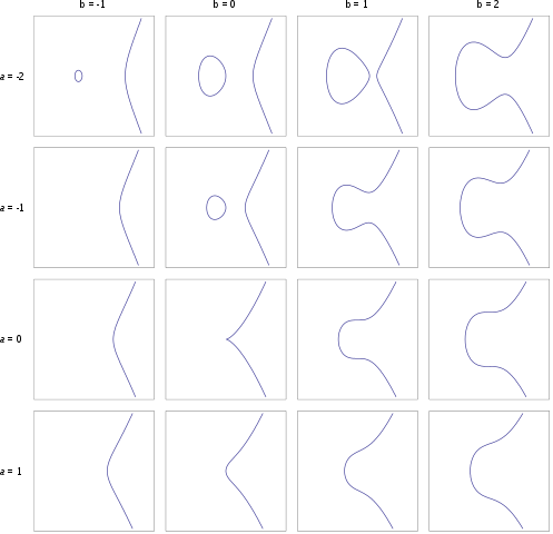
The problem with this is that it is an elliptic curve defined over the real numbers, $\Bbb{R}$. An implementation of ECC using real numbers would generally be inefficient and could further be insecure. This is where our finite field comes in:

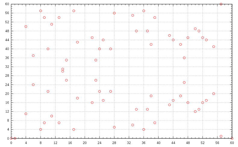
This plot is a lot less aestheticcally pleasing than the former, but better represents how elliptic curves are used in cryptography. In this case the curve is defined over the Finite Field $\Bbb{Z}_{61}$.

We could take a long detour here understanding just what Groups, Rings and Fields are (if you have the inclination then there are a number of good resources), but for our purposes I’ll just take you back to some good old fashioned maths.

Before studying the advanced topics of Trigonometry, Geometry and Algebra at school you may well have studied a number line. Most likely you would have used a line that was big enough to incorprate whatever calculations you were asked to complete. You would add (and multiply) by counting up to the right and subtract by counting down to the left. Did you ever fall off the number line? I expect not, but what if there were a fixed number of entries on the line, from $0$ to $n - 1$, and if you added too large a number and dropped off the right hand end then you simply looped back and started counting from $0$ again? The same applies if you subtract too large a number and go past $0$, you simply loop back around to the largest number on the line, $n - 1$, and carry on counting down. What I’ve just described is integer maths modulo some number, $n$. In mathematical notation this is normally referred to as $\Bbb{Z}_n$ and is known as a commutative ring.

So just where does our finite field come in?

If we take the simplest commutative ring above, $\Bbb{Z}_2$, we can draft a table of how the classic mathematical operations of addition and multiplication behave for each possible value in the set:

$\begin{array}{ccccccccccccccccccccc} \Bbb{Z}_2^+ & & 0 & 1 & & & & & & & & & & & & & & & & &\Bbb{Z}_2^\times & & 0 & 1 \\ \\ 0 & & \textcolor{#bfbfbf}{0} & \textcolor{#bfbfbf}{1} & & & & & & & & & & & & & & & & &0 & & \textcolor{#bfbfbf}{0} & \textcolor{#bfbfbf}{0} \\ 1 & & \textcolor{#bfbfbf}{1} & \textcolor{#bfbfbf}{0} & & & & & & & & & & & & & & & & &1 & & \textcolor{#bfbfbf}{0} & \textcolor{#bfbfbf}{1} \\ \end{array}$

These tables represent the addition and multiplication operations, but how could we handle subtraction? Of the 4 subtraction operations, only $0-1$ is non-trivial because it wraps around the left hand side of our number line ($-1$ is not on the line) and becomes $1$. Subtraction is just the opposite of addition, so looking back at our addition table we can use it to calculate the subtraction, reversing the steps of addition. To calculate $0-1$ simply find the $0$ in the left column and then work across the row to find $1$; The label of the column, $1$, is the result of the calculation. This technique works for any pair of values in $\Bbb{Z}_2$.

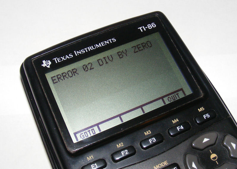
Ok, so now on to something a little harder, division. Given we only have two values, there are only 4 possible division operations $0/0$, $0/1$, $1/0$ and $1/1$. Dividing by $1$ is trivial, but dividing by $0$ presents problems! You were probably taught that dividing by $0$ isn't possible:

If we choose to ignore the challenges of dividing by 0 then the multiplication table for $\Bbb{Z}_2$ does have an answer for division in the same way the addition table also provides answers for subtraction. We can use a similar technique to above. First find the row for the denominator and then go along the row until you find the value of the numerator and then go up the column to the column header and that value gives you your result. In $\Bbb{Z}_2$ there are only two possible divisions: $0/1=0$ and $1/1=1$. This is rather simple in $\Bbb{Z}_2$, so lets move on to $\Bbb{Z}_3$:

$\begin{array}{ccccccccccccccccccccc} \Bbb{Z}_3^+ & & 0 & 1 & 2 & & & & & & & & & & & & & & & &\Bbb{Z}_3^\times & & 0 & 1 & 2 \\ \\ 0 & & \textcolor{#bfbfbf}{0} & \textcolor{#bfbfbf}{1} & \textcolor{#bfbfbf}{2} & & & & & & & & & & & & & & & &0 & & \textcolor{#bfbfbf}{0} & \textcolor{#bfbfbf}{0} & \textcolor{#bfbfbf}{0} \\ 1 & & \textcolor{#bfbfbf}{1} & \textcolor{#bfbfbf}{2} & \textcolor{#bfbfbf}{0} & & & & & & & & & & & & & & & &1 & & \textcolor{#bfbfbf}{0} & \textcolor{#bfbfbf}{1} & \textcolor{#bfbfbf}{2} \\ 2 & & \textcolor{#bfbfbf}{2} & \textcolor{#bfbfbf}{0} & \textcolor{#bfbfbf}{1} & & & & & & & & & & & & & & & &2 & & \textcolor{#bfbfbf}{0} & \textcolor{#bfbfbf}{2} & \textcolor{#bfbfbf}{1} \\ \end{array}$

Some of the values here start to get a little harder to calculate. For example $1 / 2$. How can we represent the answer to this as an integer? Normally we’d just say $0.5$ and be done, but with our example we can only work with values that are in $\Bbb{Z}_3$, i.e. $0$, $1$ and $2$. To solve this we have to restate the division problem. Rather than “What is one divided by two?” we can phrase our problem as “what value, when multiplied by two, equals one?”. Given our three options let's try each in turn:

$\begin{aligned} 0 \times 2 &= \textcolor{red}0 \\ 1 \times 2 &= \textcolor{red}2 \\ 2 \times 2 = 4 &= \textcolor{green}1 \in \Bbb{Z}_3 \end{aligned}$

And there you have your answer, $1/2$ in $\Bbb{Z}_3$ is $2$. Using our technique of finding the denominator row and then searching for the column with numerator in it also yields the correct answer. Good news!

Let’s move on to $\Bbb{Z}_4$:

$\begin{array}{cccccccccccccccccccc} \Bbb{Z}_4^+ & & 0 & 1 & 2 & 3 & & & & & & & & & & & & & &\Bbb{Z}_4^\times & & 0 & 1 & 2 & 3 \\ \\ 0 & & \textcolor{#bfbfbf}{0} & \textcolor{#bfbfbf}{1} & \textcolor{#bfbfbf}{2} & \textcolor{#bfbfbf}{3} & & & & & & & & & & && & &0 & & \textcolor{#bfbfbf}{0} & \textcolor{#bfbfbf}{0} & \textcolor{#bfbfbf}{0} & \textcolor{#bfbfbf}{0} \\ 1 & & \textcolor{#bfbfbf}{1} & \textcolor{#bfbfbf}{2} & \textcolor{#bfbfbf}{3} & \textcolor{#bfbfbf}{0} & & & & & & & & & & && & &1 & & \textcolor{#bfbfbf}{0} & \textcolor{#bfbfbf}{1} & \textcolor{#bfbfbf}{2} & \textcolor{#bfbfbf}{3} \\ 2 & & \textcolor{#bfbfbf}{2} & \textcolor{#bfbfbf}{3} & \textcolor{#bfbfbf}{0} & \textcolor{#bfbfbf}{1} & & & & & & & & & & && & &2 & & \textcolor{#bfbfbf}{0} & \textcolor{#bfbfbf}{2} & \textcolor{#bfbfbf}{0} & \textcolor{#bfbfbf}{2} \\ 3 & & \textcolor{#bfbfbf}{3} & \textcolor{#bfbfbf}{0} & \textcolor{#bfbfbf}{1} & \textcolor{#bfbfbf}{2} & & & & & & & & & & && & &3 & & \textcolor{#bfbfbf}{0} & \textcolor{#bfbfbf}{3} & \textcolor{#bfbfbf}{2} & \textcolor{#bfbfbf}{1} \\ \end{array}$

Trying to calculate $2/2$ should be simple, right? Traditional maths would tell you this is $1$, but if we again use the lookup technique and travel across the row you'll notice that both $1$ and $3$ are possible answers. This makes sense if we also flip the question around: what do you multiply by $2$ to get $2$ in $\Bbb{Z}_4$:

$\begin{aligned} 1 \times 2 &= 2 \\ 2 \times 2 = 4 &= 0 \in \Bbb{Z}_4 \end{aligned}$

Now how about $1 / 2$? If we use the lookup technique unfortunately we hit a blank, there is no $1$ value in the 3rd row (neither is there a $3$). This implies that multiplication is not invertible and so fails the Multiplicative Inverse element rule of a field.

From this we can summise that $\Bbb{Z}_2$ and $\Bbb{Z}_3$ are both finite fields, but $\Bbb{Z}_4$ is not (merely just a commutative ring!).

Does this mean that no other values will work? Well looking at the multiplication table for $\Bbb{Z}_5$:

$\begin{array}{cccccccccccccccccccc} \Bbb{Z}_5^+ & & 0 & 1 & 2 & 3 & 4 & & & & & & & & & & & & &\Bbb{Z}_5^\times & & 0 & 1 & 2 & 3 & 4 \\ \\ 0 & & \textcolor{#bfbfbf}{0} & \textcolor{#bfbfbf}{1} & \textcolor{#bfbfbf}{2} & \textcolor{#bfbfbf}{3} & \textcolor{#bfbfbf}{4} & & & & & & & & & & & & &0 & & \textcolor{#bfbfbf}{0} & \textcolor{#bfbfbf}{0} & \textcolor{#bfbfbf}{0} & \textcolor{#bfbfbf}{0} & \textcolor{#bfbfbf}{0} \\ 1 & & \textcolor{#bfbfbf}{1} & \textcolor{#bfbfbf}{2} & \textcolor{#bfbfbf}{3} & \textcolor{#bfbfbf}{4} & \textcolor{#bfbfbf}{0} & & & & & & & & & & & & &1 & & \textcolor{#bfbfbf}{0} & \textcolor{#bfbfbf}{1} & \textcolor{#bfbfbf}{2} & \textcolor{#bfbfbf}{3} & \textcolor{#bfbfbf}{4} \\ 2 & & \textcolor{#bfbfbf}{2} & \textcolor{#bfbfbf}{3} & \textcolor{#bfbfbf}{4} & \textcolor{#bfbfbf}{0} & \textcolor{#bfbfbf}{1} & & & & & & & & & & & & &2 & & \textcolor{#bfbfbf}{0} & \textcolor{#bfbfbf}{2} & \textcolor{#bfbfbf}{4} & \textcolor{#bfbfbf}{1} & \textcolor{#bfbfbf}{3} \\ 3 & & \textcolor{#bfbfbf}{3} & \textcolor{#bfbfbf}{4} & \textcolor{#bfbfbf}{0} & \textcolor{#bfbfbf}{1} & \textcolor{#bfbfbf}{2} & & & & & & & & & & & & &3 & & \textcolor{#bfbfbf}{0} & \textcolor{#bfbfbf}{3} & \textcolor{#bfbfbf}{1} & \textcolor{#bfbfbf}{4} & \textcolor{#bfbfbf}{2} \\ 4 & & \textcolor{#bfbfbf}{4} & \textcolor{#bfbfbf}{0} & \textcolor{#bfbfbf}{1} & \textcolor{#bfbfbf}{2} & \textcolor{#bfbfbf}{3} & & & & & & & & & & & & &4 & & \textcolor{#bfbfbf}{0} & \textcolor{#bfbfbf}{4} & \textcolor{#bfbfbf}{3} & \textcolor{#bfbfbf}{2} & \textcolor{#bfbfbf}{1} \\ \end{array}$

We see unique values in every row and column (apart from the first row), so based on what we’ve understood so far this means that division does work for every pair of value where the denominator is non-zero and so $\Bbb{Z}_5$ is also a finite field.

Interesting, what about $\Bbb{Z}_6$?

$\begin{array}{ccccccccccccccccccc} \Bbb{Z}_6^+ & & 0 & 1 & 2 & 3 & 4 & 5 & & & & & & & & & & &\Bbb{Z}_6^\times & & 0 & 1 & 2 & 3 & 4 & 5 \\ \\ 0 & & \textcolor{#bfbfbf}{0} & \textcolor{#bfbfbf}{1} & \textcolor{#bfbfbf}{2} & \textcolor{#bfbfbf}{3} & \textcolor{#bfbfbf}{4} & \textcolor{#bfbfbf}{5} & & & & & & & & & & &0 & & \textcolor{#bfbfbf}{0} & \textcolor{#bfbfbf}{0} & \textcolor{#bfbfbf}{0} &\textcolor{#bfbfbf}{0} & \textcolor{#bfbfbf}{0} & \textcolor{#bfbfbf}{0} \\ 1 & & \textcolor{#bfbfbf}{1} & \textcolor{#bfbfbf}{2} & \textcolor{#bfbfbf}{3} & \textcolor{#bfbfbf}{4} & \textcolor{#bfbfbf}{5} & \textcolor{#bfbfbf}{0} & & & & & & & & & & &1 & & \textcolor{#bfbfbf}{0} & \textcolor{#bfbfbf}{1} & \textcolor{#bfbfbf}{2} &\textcolor{#bfbfbf}{3} & \textcolor{#bfbfbf}{4} & \textcolor{#bfbfbf}{5} \\ 2 & & \textcolor{#bfbfbf}{2} & \textcolor{#bfbfbf}{3} & \textcolor{#bfbfbf}{4} & \textcolor{#bfbfbf}{5} & \textcolor{#bfbfbf}{0} & \textcolor{#bfbfbf}{1} & & & & & & & & & & &2 & & \textcolor{#bfbfbf}{0} & \textcolor{#bfbfbf}{2} & \textcolor{#bfbfbf}{4} &\textcolor{#bfbfbf}{0} & \textcolor{#bfbfbf}{2} & \textcolor{#bfbfbf}{4} \\ 3 & & \textcolor{#bfbfbf}{3} & \textcolor{#bfbfbf}{4} & \textcolor{#bfbfbf}{5} & \textcolor{#bfbfbf}{0} & \textcolor{#bfbfbf}{1} & \textcolor{#bfbfbf}{2} & & & & & & & & & & &3 & & \textcolor{#bfbfbf}{0} & \textcolor{#bfbfbf}{3} & \textcolor{#bfbfbf}{0} &\textcolor{#bfbfbf}{3} & \textcolor{#bfbfbf}{0} & \textcolor{#bfbfbf}{3} \\ 4 & & \textcolor{#bfbfbf}{4} & \textcolor{#bfbfbf}{5} & \textcolor{#bfbfbf}{0} & \textcolor{#bfbfbf}{1} & \textcolor{#bfbfbf}{2} & \textcolor{#bfbfbf}{3} & & & & & & & & & & &4 & & \textcolor{#bfbfbf}{0} & \textcolor{#bfbfbf}{4} & \textcolor{#bfbfbf}{2} &\textcolor{#bfbfbf}{0} & \textcolor{#bfbfbf}{4} & \textcolor{#bfbfbf}{2} \\ 5 & & \textcolor{#bfbfbf}{5} & \textcolor{#bfbfbf}{0} & \textcolor{#bfbfbf}{1} & \textcolor{#bfbfbf}{2} & \textcolor{#bfbfbf}{3} & \textcolor{#bfbfbf}{4} & & & & & & & & & & &5 & & \textcolor{#bfbfbf}{0} & \textcolor{#bfbfbf}{5} & \textcolor{#bfbfbf}{4} &\textcolor{#bfbfbf}{3} & \textcolor{#bfbfbf}{2} & \textcolor{#bfbfbf}{1} \\ \end{array}$

Unfortunately, like $\Bbb{Z}_4$, $\Bbb{Z}_6$ also has values that have no multiplicative inverse, so not a finite field.

Although we’ve only looked at a small handful of $\Bbb{Z}_i$s here you might have noticed a pattern; $\Bbb{Z}_i$ is a finite field when $i$ is prime number. Consider writing out further tables as an exercise for the reader, but this pattern continues for all (the infinite number of) primes.

In this post you have learnt how to do basic math operations in a Finite Field, carry on to part 2 to look at more complex operations and non-prime fields.